Create 3D (XYZC) grids in Surfer

3D volumetric modeling provides essential insights for analyzing complex spatial data, such as groundwater contamination, soil chemistry, or subsurface geology. Creating 3D grid files (XYZC) in Surfer enables you to visualize and evaluate 3D volumes, isosurfaces, contours, slices, and drillhole data with precision.

What is a 3D grid?

A 3D grid (XYZC) is a regularly spaced, three-dimensional cuboid array of nodes. While X and Y represent horizontal map coordinates and Z represents elevation or depth, C represents a variable value assigned to each X, Y, Z location—such as contaminant concentration, soil density, or temperature.

How to create a 3D grid from XYZC point data

Generating an XYZC 3D grid file in Surfer follows a similar workflow to traditional 2D surface gridding:

1. Click Home | Grid Data | Grid Data.
2. In the Grid Data - Select Data dialog:
   1. Select XYZC in the Data Type section.
   2. Choose your preferred Gridding Method.
   3. Click Browse in the Dataset 1 field, select your XYZC data file, and click Open.
   4. Assign the appropriate X, Y, Z, and C data columns and click Next.
3. In the Grid Data - Options dialog, adjust search neighborhoods, anisotropy, or math parameters as needed, then click Next.
4. In the Grid Data - Output dialog:
   1. Adjust the grid spacing, limits, and NoData settings as desired.
   2. Click the folder icon in the Output Grid field to name and save your 3D grid file (`.3dv`).
   3. Select your preferred output New layer type and click Finish.

How to create a 3D grid from drillhole data

The most efficient way to grid subsurface drillhole or well data is to create a Drillhole map layer first. This allows you to visually verify interval data, logs, and paths before calculating the 3D volume model.

1. (Optional) Create a Drillhole map in Surfer to verify your data import.
2. Click Home | Grid Data | Grid Data.
3. In the Grid Data - Select Data dialog:
   1. Select Drillhole XYZC in the Data Type section.
   2. Choose your preferred Gridding Method.
   3. If you skipped step 1, click Import Drillhole Data and complete the drillhole import wizard.
   4. Click Next.
4. In the Grid Data - Options dialog, adjust parameters as needed and click Next.
5. In the Grid Data - Output dialog, specify grid limits, resolution, and output file name, then click Finish.

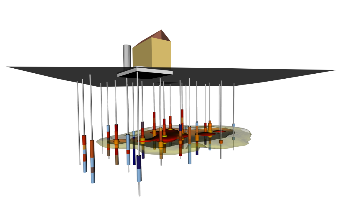
3D gridding methods

Surfer offers four specialized XYZC 3D gridding methods to accommodate different data distributions and sampling density:

• Inverse Distance to a Power: The default and most universal method for general XYZC data. It is fast and honors the actual minimum and maximum data ranges without extrapolating beyond the data boundaries. You can apply Anisotropy settings to weight influence in preferred directions (e.g., setting X and Y lengths 10 to 100 times larger than Z length for shallow soil horizons, or smaller Z lengths for dense down-hole data).
• Nearest Neighbor: Ideal for regularly spaced XYZC point datasets or direct equipment readings where no interpolation is required. Nearest Neighbor assigns the value of the nearest point to each grid node. To maintain data accuracy, ensure X, Y, and Z grid spacing matches your exact data point intervals.
• Local Polynomial: Best suited for datasets that exhibit local smoothness within defined search neighborhoods. Because processing speed is not significantly impacted by dataset size, it serves as an excellent fast method for massive 3D point datasets.
• Data Metrics: Calculates statistical information about your data distribution (such as point counts or distance to points per node). This method is primarily used for quality control and data density evaluation rather than property modeling.

Additional Resources

• Best practices for gridding drillhole data
• Create Interactive 3D Site Models with Surfer (webinar)