Gridding, also known as data interpolation, is the process of converting scattered, real-world data points into a continuous, evenly spaced grid. This process is analogous to adding a fit curve to a 2D scatter plot. While a fit curve models the trend between X and Y data points along a line, gridding expands this concept into three dimensions by fitting a continuous surface to your XYZ data or a matrix to your XYZC data.
Just as you would choose between a simple straight line or a complex curve to accurately represent your scatter plot's trend, there are many different gridding methods available to create a surface. Each method uses a unique mathematical algorithm. Some are excellent for creating smooth, flowing surfaces like those seen in elevation or temperature maps. Others are better at preserving sharp edges and abrupt changes, which are common in fields like geology or environmental analysis.
Choosing the right gridding method is one of the most critical steps in data analysis. The method you select directly controls the appearance and, more importantly, the accuracy of your final map. An inappropriate choice can distort your results—much like using a straight line to model a curved dataset—leading to a flawed interpretation of your data. This article will help you understand the gridding methods available in Surfer so you can choose the best one for your needs and create the most accurate and meaningful map possible.
For more specific guidance on how to test which gridding method is best for your data, see Choosing the right gridding method in Surfer
| Surfer gridding methods covered in this article: |
Kriging
Kriging is one of the more flexible and accurate gridding methods and is therefore the method that is most often recommended. Kriging is effective because it produces a good map for most data sets and it can compensate for clustered data by giving less weight to the cluster in the overall prediction. One of the disadvantages to Kriging is that it can be slower than other methods, especially when working with large data sets. It also often extrapolates grid Z values beyond the range of the input data’s Z values.
| The classed post map, left, represents scattered elevation data that produced the contour map, right, using the Kriging gridding method. |
How kriging works
Each grid node value is based on the known data points neighboring the node. Each data point is weighted by its distance away from the node. This way, points that are further from the node will have less weight in the estimation of the node. For example, to compute the Z value at grid node A, this equation is used:
Where ZA is the estimated value of grid node A, n is the number of neighboring data values used in the estimation, Zi is the value at location i with weight, Wi. The value of weights will sum to 1 to make sure there is no bias towards clustered data points. The formula can get more complex if things such as drifts and a search radius are applied.
Gridding data using Kriging in Surfer
In Surfer, default properties of Kriging are point Kriging with no drifts and a circular search ellipse. The default properties are used unless otherwise specified.
- Click Home | Grid Data | Grid Data.
| Select Kriging under Gridding Method in the Grid Data - Select Data dialog. |
- In the Grid Data - Select Data dialog, change the Gridding Method to Kriging.
- Click Browse to select your Dataset.
- Set the X, Y, and Z columns and click the Next button to select a variogram model.
- The Grid Data - Kriging - Variogram dialog provides all of the properties needed to select the appropriate variogram model for your data.
A variogram is a description of the surface’s roughness based quantitatively and statistically. The variogram is the degree of variance between values at two locations, x and y. This section is useful for adding components to the variogram produced with the Kriging gridding method. For example, a nugget can be added to the variogram, which represents a jump at the origin for the semivariogram. If you are not sure what components to add, it is best to use the default Linear variogram, with no nugget effect. For more information on variograms, see Variogram modelling for kriging in Surfer - a tutorial.
| The Grid Data - Kriging - Variogram dialog contains customizable options to best fit the Kriging gridding method to the data. |
- Click the Next button to select custom Kriging options.
- The Grid Data -Kriging - Options dialog has three different sections that contain specialized customization options. Detailed information about each section can be found in Surfer's help:
| The Grid Data - Options dialog contains customizable options to best fit the Kriging gridding method to the data. |
- Click Next to view the cross validation report.
- Click Next to view the output grid options.
| The Grid Data - Output dialog contains customizable options for finishing your grid file such as adjusting the resolution and assigning NoData. |
- On the Grid Data - Kriging - Output dialog:
- Increase the resolution of your output grid by adjusting the Spacing or # of Nodes in the X Direction and Y Direction.
- Assign a null or NoData value to certain areas using the Assign NoData outside of options or by defining a NoDataPolygon Boundary.
- Define a file name, format, and location in the Output Grid field.
- Select how and where you'd like your grid file displayed using the Add grid as layer to and New layer fields.
- Click Finish to create your grid file.
Nearest Neighbor
Nearest Neighbor is best used with regularly spaced data points. If the observations have a few missing data points, this method is best for filling in the holes. This method is an exact interpolator and does not extrapolate beyond the Z range of the data.
| The classed post map, left, was created with the data points. The contour map, left, represents the interpolated grid nodes using the Nearest Neighbor gridding method. |
How nearest neighbor works
The Nearest Neighbor method is not mathematically intense. When using Nearest Neighbor, the Z value of each grid node is simply the Z value of the nearest original data point to that grid node. The nearest neighbor to a grid node uses a simple separation distance without taking anisotropy into account. If two or more points tie as the nearest neighbor, the tied data points are sorted on X, then Y, and then Z values. The smallest value is selected as the nearest neighbor.
Nearest neighbor options in Surfer
To set the gridding method to Nearest Neighbor, in the Grid Data - Select Data dialog, change the Gridding Method to Nearest Neighbor, select your Dataset, and set the X, Y, and Z columns. To customize Nearest Neighbor, click the Next button to bring up the Grid Data - Nearest Neighbor - Options dialog.
 |
| Click the Next button to open the Grid Data - Nearest Neighbor Options dialog. |
The Search section allows you to specify the radii and angles of the search ellipse.
| The Search section contains the settings for the search ellipse. |
- The search ellipse specifies the size of the local neighborhood in which to look for data, this can be impacted by the search rules set. The values of radius 1 and radius 2 are the distance in positive data units. The radii values are the lengths that are searched in the direction indicated by the angle. The angle is represented in orientation between the positive x axis and the radius 1 of the ellipse axis. If there are no points found in the search ellipse then that grid node will be assigned the NoData value. By default, the search ellipse is circular giving equal weight to both directions surrounding the grid node. The default length is the diagonal distance of the data.
The search options can be customized so that large areas that have no data points are assigned the NoData value. To do this, set the radius of the search ellipse equal to a value that is less than the distance between data values.
The Breaklines and Faults section allows for you to specify the boundary files for the breaklines and faults to be used in gridding.
|
The Breaklines and Faults section is used to upload a blanking file with the breaklines and faults information. |
- A breakline is an interruption in a surface’s slope that is often wavy and irregular, such as the base of a cliff. These are useful to represent any irregularities and disconformities in the map. Breaklines are not barriers when gridding; this means that all data points on both sides of the line are used when interpolating the grid nodes, regardless of the position on either side of the line. However, if a grid node is located on the boundary line then the value of the grid node becomes the value of the boundary file.
The breakline file contains the X, Y, and Z vertices of the interruption in a blanking file (*.BLN) format: the first row is the number of data points in the file followed by the XYZ coordinates of the line. - A fault is a 2D line that acts as a barrier when gridding data. The fault lines represent a significant discontinuity along fractures due to the movement of the earth. In gridding, the fault line acts as a barrier of information when gridding. The data on one set of the fault is not used when interpolating the values on the other side of the fault line.
A fault file contains the X and Y values of the line that represent the fault in a blanking file (*.BLN) format: the first row is the number of data points in the file followed by the XY coordinates of the line.
Natural Neighbor
The natural neighbor gridding method is popular with data sets that have dense data in some areas and sparse data in other areas. The Natural Neighbor estimates the grid node value by finding the closest subset of input data points to a grid node and then applying weight to each. The Natural Neighbor method does not extrapolate the Z grid values beyond the range of data and it does not generate nodes in areas without data.
| The classed post map, left, was created with the data points. The contour map, left, represents the interpolated grid nodes using the Natural Neighbor gridding method. |
Natural neighbor options in Surfer
The Natural Neighbor method has options to set the anisotropy and to save the Delaunay triangles. To specify the advanced options of the Natural Neighbor gridding method, in the Grid Data - Select Data dialog, click the Next button.
| Click the Advanced Options button to open the Grid Data Advanced Options dialog. |
Anisotropy is useful in eliminating trends in the data when interpolating the grid nodes. Anisotropy refers to directionally dependent data. The Grid Data Advanced Options dialog allows you to specify three different customizations of the gridding. The customizable areas:
| The Grid Data - Natural Neighbor - Options allows the anisotropy settings to be specified when gridding the data. |
- Anisotropy Ratio: This value defines the relative weight of the points when interpolating the grid nodes. This value is computed by dividing the maximum range by the minimum range. For most data sets, it is recommended to accept the default value of 1, which means that all points have the same weight. You may want to increase the ratio of the points in one direction that has more similarity than the points in another direction. By increasing the ratio, the points in the direction defined will have more weight on the value of the interpolated grid node. The ratio is typically considered severe if greater than four and mild if less than two.
- Anisotropy Angle: The angle is the direction of the major axis, in degrees. The angle rotates counterclockwise with 0 degrees being east-west and 90 degrees being north-south going multiple directions. In order to use a direction angle, an anisotropy angle should not equal 1.
- Save Triangles To: The Delaunay triangles are formed by connecting lines between data points. Often the triangles are formed by maximizing the minimum angle; this prevents small triangles from being formed. The result is triangular faces all over the grid. If two or points are located on the same line then there is no Delaunay triangulation. The triangles that are formed are not intersected by other triangles. The triangles can be useful to determine the density of the data points. The Delaunay triangles can be loaded as a base map and combined with other maps. To save the file, click the folder icon and specify the location and file format to save the file.
Local Polynomial
Local polynomial interpolation works best with data sets that are relatively smooth within search neighborhoods. This method fits an ordered polynomial using points within a defined neighborhood. The different polynomials allows for different fits through the data. For example, a single-order polynomial fits a plane through the data; a second-order fits a surface with a bend; a third-order accommodates two bends, and so on. If the surface being gridded has multiple shapes, such as repetitive sloping and leveling then it is best to use multiple polynomial planes. The multiple polynomial planes would represent the surface more accurately. This method is useful with larger data sets because the computation speed is not affected by the data set size.
A polynomial equation is fit against the data using weighted least squares. The grid nodes are assigned the value of the polynomial at each node. Surfer allows the polynomials to be of order 1, 2, or 3. The data that is closer to the grid node has a higher weight than the data that is further away.
The example below shows a data set that was gridded using the Local Polynomial gridding method.
| The classed post map, left, was created with the data points. The contour map, left, represents the interpolated grid nodes using the Local Polynomial gridding method. |
Local polynomial options in Surfer
To specify the advanced options of the Local Polynomial gridding method, in the Grid Data dialog, click Advanced Options.
| Click the Next button to open the Grid Data - Select Data dialog. |
The Local Polynomial Parameters section of the Grid Data - Local Polynomial Options displays the Power and Polynomial Order properties.
| The General section in the Grid Data Advanced Options dialog is used to customize the power and polynomial order of the gridding method. |
- Power: The power specified is applied to the weight calculation that is used to minimize the sum of the squared residuals. Set the power to a value between 0 and 20.
- Polynomial Order: This allows you to select the order of the polynomial that you would like to use to interpolate the data.
The Search Neighborhood section allows you to specify the search options of which points are considered when interpolating grid nodes.
 |
| The Search Neighborhood section contains setting to modify the search parameters of the selected gridding method. |
-
Search options: The options set in the SearchNeighborhood allow Surfer to know which data points to use when interpolating the grid nodes. It can be useful to specify the search settings for different types of data sets, such as different sizes of data sets.
- Number of sectors to search: Allows the search area to be divided into sections, up to 32 search sectors can be specified. This is ideal for data that is clustered.
- Maximum number of data to use for ALL sectors: This limits the total number of points used in the overall estimation.
- Maximum number of data to use from EACH sector: This value dictates the number of points to be used from each sector.
- Minimum number of data in all sectors (node is set to NoData if fewer): If there are not enough points found when estimating a grid node then Surfer will assign that grid node the NoData value. The grid nodes with NoData values represent insufficient data and will trim the contour lines on the map.
- Assign NoData to node if more than this many sectors are empty: If there are not enough sectors for the grid node then Surfer will assign that grid node the NoData value.
- Search Ellipse: The search ellipse specifies the size of the local neighborhood in which to look for data, this can be impacted by the search rules set. The values of radius 1 and radius 2 are the distance in positive data units. The radii values are the lengths that are searched in the direction indicated by the angle. The angle is represented in orientation between the positive x axis and the radius 1 of the ellipse axis. If there are no points found in the search ellipse then that grid node will be assigned the NoData value. By default, the search ellipse is circular giving equal weight to both directions surrounding the grid node. The default length is half the diagonal distance of the data.
The search options can be customized so that large areas that have no data points are assigned the NoData value. To do this, set the radius of the search ellipse equal to a value that is less than the distance between data values.
The Breaklines section allows for you to specify the boundary files for the breaklines to be used in gridding.
| The Breaklines section is used to upload a blanking file with the breaklines information. |
- A breakline is an interruption in a surface’s slope that is often wavy and irregular, such as the base of a cliff. These are useful to represent any irregularities and disconformities in the map. Breaklines are not barriers when gridding; this means that all data points on both sides of the line are used when interpolating the grid nodes, regardless of the position on either side of the line. However, if a grid node is located on the boundary line then the value of the grid node becomes the value of the boundary file.
The breakline file contains the X, Y, and Z vertices of the interruption in a blanking file (*.BLN) format: the first row is the number of data points in the file followed by the XYZ coordinates of the line.
Radial Basis Function
The Radial Basis Function gridding method is an exact interpolator which means your data is honored. The real-value function depends on the distance from the origin. This method is similar to Kriging in that it is flexible and it generates an accurate interpretation of most data sets. The method can handle large sets of data and produce a smooth surface. However this is not an ideal method if the data has large changes in surface values within short distances. The Radial Basis Function method takes the user-specified function and fits it through the data values.
The example below shows a data set that was gridded using the Radial Basis Function gridding method.
| The classed post map, left, was created with the data points. The contour map, left, represents the interpolated grid nodes using the Radial Basis Function gridding method. |
Radial basis function options in Surfer
To specify the advanced options of the Radial Basis Function gridding method, in the Grid Data - Select Data dialog, click the Next button.
| Click the Next button to open the Grid Data - Radial Basis Function - Options dialog. |
The Radial Basis Parameters section allows you to specify the Basis Function and R2 Parameter.
| The Radial Basis Parameters section contains some of the customizable settings for the gridding method. |
-
Basis Function: Allows you to specify the function basis. The function chosen defines the optimal set of weights to apply to the data points when interpolating a grid node. The types of functions have the following equations:
The functions above represent the functions that can be
selected as the Basis Function for the gridding method. -
R2 Parameter: R2 is referred to as the shaping factor. A larger R2 value will produce a map with smooth contour lines and round mountain tops. The value is calculated using this formula:
(length of diagonal of the data extent)2 / (25 * number of data points)
The Radial Basis Function is an exact interpolator, no matter what value is entered for R2. -
Anisotropy Ratio: This value defines the relative weight of the points when interpolating the grid nodes. This value is computed by dividing the maximum range by the minimum range. For most data sets, it is recommended to accept the default value of 1, which means that all points have the same weight. You may want to increase the ratio of the points in one direction that has more similarity than the points in another direction. By increasing the ratio, the points in the direction defined will have more weight on the value of the interpolated grid node. The ratio is typically considered severe if greater than four and mild if less than two.
Anisotropy Angle: The angle is the direction of the major axis, in degrees. The angle rotates counterclockwise with 0 degrees being east-west and 90 degrees being north-south going multiple directions. In order to use a direction angle, an anisotropy angle should not equal 1.
The Search Neighborhood section allows you to specify the search options of which points are considered when interpolating grid nodes.
| The Search Neighborhood section contains setting to modify the search parameters of the selected gridding method. |
-
Search options: The options set in the Search tab allow Surfer to know which data points to use when interpolating the grid nodes. It can be useful to specify the search settings for different types of data sets, such as different sizes of data sets. For example, if the data set is small (under 250 data points) then it is more reasonable to use the No Search option and interpolate the grid nodes with all of the data. On the contrary, if the data set is large then it may be ideal to limit the number of data points used to interpolate each grid node.
- No Search: When this option is selected then Surfer will use all of the data points in estimating the grid file. This is useful for smaller data sets, up to 250 points. This is also adequate for evenly distributed data. If this option is disabled, it is because there are more than 750 data points and Surfer cannot grid the data without breaking the file into smaller sectors.
- Number of sectors to search: Allows the search area to be divided into sections, up to 32 search sectors can be specified. This is ideal for data that is clustered.
- Maximum number of data to use for ALL sectors: This limits the total number of points used in the overall estimation.
- Maximum number of data to use from EACH sector: This value dictates the number of points to be used from each sector.
- Minimum number of data in all sectors (node is set to NoData if fewer): If there are not enough points found when estimating a grid node then Surfer will assign that grid node the NoData value. The grid nodes with NoData values represent insufficient data and will trim the contour lines on the map.
- Assign NoData to node if more than this many sectors are empty: If there are not enough sectors for the grid node then Surfer will assign that grid node the NoData value.
- Search Ellipse: The search ellipse specifies the size of the local neighborhood in which to look for data, this can be impacted by the search rules set. The values of radius 1 and radius 2 are the distance in positive data units. The radii values are the lengths that are searched in the direction indicated by the angle. The angle is represented in orientation between the positive x axis and the radius 1 of the ellipse axis. If there are no points found in the search ellipse then that grid node will be assigned the NoData value. By default, the search ellipse is circular giving equal weight to both directions surrounding the grid node. The default length is half the diagonal distance of the data.
The search options can be customized so that large areas that have no data points are assigned the NoData value. To do this, set the radius of the search ellipse equal to a value that is less than the distance between data values.
The Breaklines section allows for you to specify the boundary files for the breaklines to be used in gridding.
| The Breaklines section is used to upload a blanking file with the breaklines information. |
- A breakline is an interruption in a surface’s slope that is often wavy and irregular, such as the base of a cliff. These are useful to represent any irregularities and disconformities in the map. Breaklines are not barriers when gridding; this means that all data points on both sides of the line are used when interpolating the grid nodes, regardless of the position on either side of the line. However, if a grid node is located on the boundary line then the value of the grid node becomes the value of the boundary file.
The breakline file contains the X, Y, and Z vertices of the interruption in a blanking file (*.BLN) format: the first row is the number of data points in the file followed by the XYZ coordinates of the line.
Triangulation with Linear Interpolation
The Triangulation with Linear Interpolation works best with data that is evenly distributed over the grid area. If the map is produced with triangular facets then the data set may be too small or most likely contains sparse areas. The gridding method draws lines between data points to create triangles, none of the triangle edges are intersected by other triangles. This gridding method is fast and does not extrapolate beyond the Z value of the data range. In addition, Triangulation with Linear Interpolation does not create data that is outside the data limits; it assigns the NoData value to the grid nodes that are outside the data limits.
The example below shows a data set that was gridded using the Triangulation with Linear Interpolation gridding method.
| The classed post map, left, was created with the data points. The contour map, left, represents the interpolated grid nodes using the Triangulation gridding method. |
Triangulation with linear interpolation options in Surfer
To specify the advanced options of the Triangulation with Linear Interpolation gridding method, in the Grid Data - Select Data dialog, click the Next button.
| Click the Next button to open the Grid Data - Select Data dialog. |
Anisotropy is useful in eliminating trends in the data when interpolating the grid nodes. Anisotropy refers to directionally dependent data. The Grid Data Advanced Options dialog allows you to specify three different customizations of the gridding. The customizable areas:
| The Grid Data - Triangulation with Linear Interpolation - Options dialog allows the anisotropy settings to be specified when gridding the data. |
- Anisotropy Ratio: This value defines the relative weight of the points when interpolating the grid nodes. This value is computed by dividing the maximum range by the minimum range. For most data sets, it is recommended to accept the default value of 1, which means that all points have the same weight. You may want to increase the ratio of the points in one direction that has more similarity than the points in another direction. By increasing the ratio, the points in the direction defined will have more weight on the value of the interpolated grid node. The ratio is typically considered severe if greater than four and mild if less than two.
- Anisotropy Angle: The angle is the direction of the major axis, in degrees. The angle rotates counterclockwise with 0 degrees being east-west and 90 degrees being north-south going multiple directions. In order to use a direction angle, an anisotropy angle should not equal 1.
- Save Triangles To: The Delaunay triangles are formed by connecting lines between data points. Often the triangles are formed by maximizing the minimum angle; this prevents small triangles from being formed. The result is triangular faces all over the grid. If two or points are located on the same line then there is no Delaunay triangulation. The triangles that are formed are not intersected by other triangles. The triangles can be useful to determine the density of the data points. The Delaunay triangles can be loaded as a base map and combined with other maps. To save the file, click the folder icon and specify the location and file format to save the file.
Data Metrics
The Data Metrics gridding method can be used to map statistical parameters of a data set. Although Data Metrics is a gridding method, it is different than most because it does not interpolate the data to obtain a Z value. Data Metrics is used to gain information about data points in the form a grid. It is recommended to use the same settings (i.e. grid line geometry, search, breakline, and fault parameters) as you would when gridding with another method.
There are five major groups of the Data Metrics gridding method: Z order Statistics, Z Moment Statistics, Other Z Statistics, Data Location Statistics, and Terrain Statistics. Each group is categorized based on the detail it is analyzing of the data. For each statistical parameter, the data is divided into search sections where the calculation will be performed. The value returned for the calculation will then be assigned to the grid node in that region. Data metrics allows you to define the size and specific nodes for each search parameter. This method is useful when determining specific information about the data that was calculated and created maps from those calculations.
Z Order Statistics
The Z Order Statistics provide specific statistical information about the data that is specified within the search radius. The Z grid node values will have the same units as the original data file. These data values can be significant to calculate if the goal is to demonstrate areas of statistical interest. The data that is found in the search radius will be sorted from least to greatest and then the following statistics can be calculated.
| The image above shows a sorted set of data and the appropriate data metrics that are calculated based on the data. |
- Minimum: The Minimum is calculated by returning the first result of the sorted data in the search parameters. An application of this gridding method would be to show the areas of lowest elevation in comparison to surrounding areas to represent the areas with the highest rate of erosion.
- Median: The median is the middle value in the data set. The median value can be useful if the data is skewed to one direction, thus leaving the average to be skewed as well. The median is a good measure of the middle value in a set of data, such as a grid of the middle points in the Rocky Mountains. Using the median will allow for the outliers not to be taken into account so the grid would be an accurate representation of the middle peaks.
- Maximum: The Maximum value is determined by returning the last value in the sorted data. This statistical representation can be useful when creating a canopy map of the forest that represents the greatest heights of the trees.
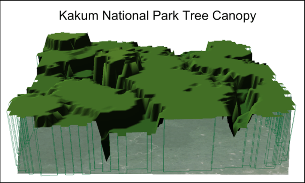 |
| The Kakum National Park Tree Canopy grid, shown above as a 3D Surface, represents that tallest trees in the Kakum National Park, Ghana. The data used in the image is fictional and used to demonstrate an application of the Maximum statistical value. |
- Range: The range of the data is taken by subtracting the minimum value from the maximum value. This value can be useful to determine the difference between the values that are located in each search section. An application of this method includes creating a grid file to represent the elevations used when creating a contour plot to verify the accuracy.
- MidRange: The midrange value is the half the value of the sum of the maximum and the minimum. The value can be more applicable than the median, since it takes into account the data range instead of the location of the middle number. The midrange value represents the true middle of the data range.
| The model above displays a full data set, at the top, and then it split into the upper and lower half based on the median value, 8. The median is then taken of the upper and lower half to return the upper and lower quartile values, respectively. |
- Lower Quartile: The data is divided into half, and the median of the lower half is returned. The value returned will represent the lower 25% of the data. The lower quartile can provide insight on which the range of the lower outliers exists.
- Upper Quartile: The data is divided into half, and the median of the upper half is returned. The value returned will represent the upper 25% of the data. The upper quartile can provide insight on which the range of the upper outliers exists.
- Interquartile Range: The interquartile range is the lower quartile subtracted from the upper quartile. The difference can be used to show the spatial variability. Since the data focus mostly on the center data, it does not take into account the distributions at the end of the data. The interquartile range can provide insight as to where most of the data lies since the outliers have been removed.
Z Moment Statistics
The Z moment statistics use the data that is specified in the search radius to perform specific statistical calculations about the values in the node. The statistic values show the variability in the data set and how the values relate to one another. The grid node value assigned at the grid is in the same data units as the original Z values.
- Mean: The mean value is determined by summing up the data and then dividing by the number of points in the search section. The mean value is useful to determine the average value calculate in a specific area.
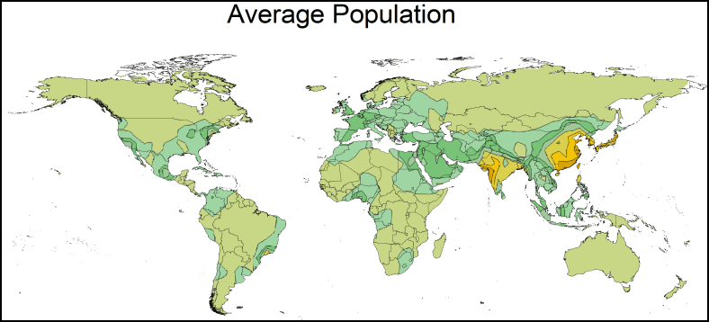 |
| The contour map created above is displaying the mean population for the world based on the mean population of the major surrounding cities. |
- Standard Deviation: This value is calculated by summing all the Z values in the search area to compute the variance, and then the square root is taken of the variance to determine the standard deviation. The standard deviation value identifies the variability of each data value from the mean. This is useful to summarize continuous data. Since this method returns values based on the mean, it is not recommended to use this method if the data set contains a high number of outliers.
- Variance: This value is the square standard deviation of the data defined in the search parameters. The variance value can depict the variability of the data. The closer the variance is the zero, the closer the data is located near the mean. When the variance value is larger, then the data is scattered. Using this method can be useful in determining where the data is the most spread out to reveal inconsistencies in the data or identify areas of concern.
- Coefficient of Variation: The coefficient of variation is the ratio between the standard deviation and the mean. This calculation is used when interested in the variability of the data compared to the observation size.
Other Z Statistics
The statistical methods listed under the Other Z Statistics are used to analyze the data without requiring the data to be sorted. The values that are calculated for each node will have the same units as the Z value in the data set.
- Sum: This value will add up all the Z values that are included in the search region. This calculation can be useful in determining the total values for a given region. For example, this can represent regions with high contamination values as shown in the plot below.
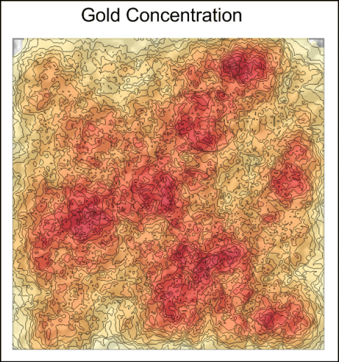 |
| The map above was created using a shaded relief map overlaid with a contour plot. The grid file was generated using the Sum statistical count to represent the areas with the highest concentration of gold. |
- M.A.D: The median absolute deviation value is calculated by determining the median in the search range and then deviations are taken for each value. Once the deviation values are determined, then the median is taken from that set and assigned as the Z value for that grid node. This method is more resilient to outliers and ideal for data sets that do not contain a median or a variance.
-
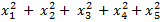
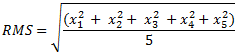
R.M.S.: The root mean square value is calculated by taking the square root of the average of all the values squared. This means, using the data set
 :
:
- The data values are squared and summed:
- The average is taken of the value from Step 1:
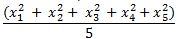
- The square root of the value in Step 2 is calculated to obtain the RMS value:
- The data values are squared and summed:
Data Location Statistics
The statistics for Data Locations are concerned with the location of the data points, unlike the methods mentioned above. The location of data points is often useful when determining the density or the distance from each other. The values calculated in the statistics are in the same units as the original data set. Since the values are not concerned about the Z value at each location, the data metrics are calculated based on the XY data points.
For example, a use of the Count Data Metrics can be represented in the map below. The grid represents the number of health care facilities per area in Kenya. This map can then be used to represent a link between the number of health care facilities and the rate of illness.
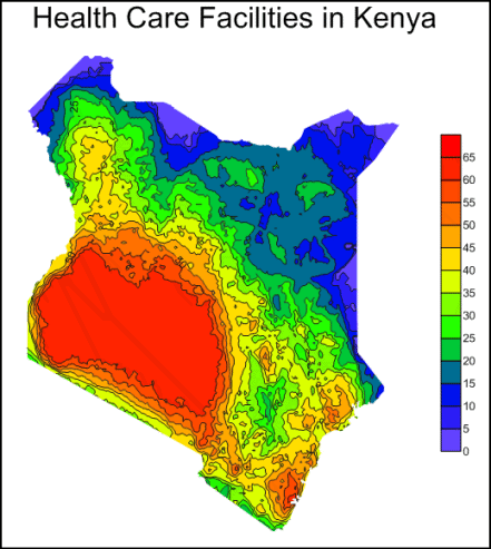 |
| The map above was created using the Count statistics to represent the number of health care facilities in the entire region of Kenya, Africa. The color scale, on the right, shows the colors that correspond to the specific Z values. |
- Count: The count value is determined by simply calculating the number of points inside the specified search area. The count of the data points in a particular area can be useful in generating a probability map to demonstrate the likeliness of an even occurring in a given location. This is often useful when determining areas of high risk or repetitive events.
- Approximate Density: Data density within the search. This can be helpful if you want to determine the number of points that are within a certain area, also known as a density map.
- Distance to Nearest: The distance returned here is the distance between the grid node and the nearest data point. This can be useful in determining which areas are more clustered in the data set.
- Distance to Farthest: The distance calculated is the distance between the grid node and the furthest data point in the search range. This can be useful in determining how spatial the data is and how far the data points being calculated are.
- Median Distance: Similar to median calculation, this value returns the median distance based on the distance values for each point in the search parameter. Using the method can return a more accurate representation of the data because it does not give much weight to outliers in the data.
- Average Distance: This is the average distance value from the grid node to the data point. This can be useful in determining the average distance between the data and the grid node.
- Offset Distance: The first thing calculated is the center location of the data points. Then the distance between that centroid and the grid node are calculated are returned as the Z value for this offset distance. This method will provide insight if the data is located near the grid node or further away.
Terrain Statistics
Similar the Grids | Calculate | Calculus commands, the Terrain Statistics will provide specific information on the slope and aspect of the grid. Using Data Metrics will allow the data to be sampled in sections instead of as an entire grid, as it is done with the Grids | Calculate | Calculus command. This will allow for a more accurate representation of the slope and aspect since the search parameters allow a single section to be focused on at a time. For example, both of the Terrain Slope and Terrain Aspect values can be used in determining the strike and dip values for the data set.
- Terrain Slope: The value returned for the slope measures the degree of inclination relative to the horizontal plane. This method is useful to calculate the slope in each search parameter and represent areas of a constant slope in a contour map. The value returned is in degrees. A possible error is this gridding method is obtaining a horizontal plane. The result of this is because the search parameters are not defined correctly for the data set. It is recommended to reduce the search radii to search a more specific area.
- Terrain Aspect: The value calculated for each search parameter is the dip of the area, or the direction which the download slope is facing. The terrain aspect value is returned in degrees and is meaningless if the slope is zero because the area is flat.
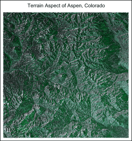 |
| The contour map above displays a grid file created using the Terrain Aspect measurement to represent Aspen, Colorado. The contour plot was exported as a KML file and displayed in Google Earth. |
Advanced Options
To specify the advanced options of the Data Metrics gridding method, in the Grid Data - Select Data dialog, select Data Metrics for the Gridding Method, set Dataset1 to your data, set the X, Y, Z columns and click Next.
| Select the data, Gridding Method and assign the columns in the Grid Data - Select Data dialog. |
The Data Metrics Parameters section of the Grid Data - Data Metrics - Options displays the statistical options to use when gridding the data.

The Search Neighborhood section allows you to specify the search options of which points are considered when interpolating grid nodes.

|
| The Search Neighborhood section contains setting to modify the search parameters of the selected gridding method. |
The Search Ellipse specifies the size of the local neighborhood in which to look for data, this can be impacted by the search rules set. The values of radius 1 and radius 2 are the distance in positive data units. The radii values are the lengths that are searched in the direction indicated by the angle. This means if trying to search an area of 5, then the search radii values should be half, 5/2 = 2.5. This value identifies to search in a circular area around the grid node with a diameter of 5m.
The Search Angle represents the orientation between the positive x axis and the radius 1 of the ellipse axis. If there are no points found in the search ellipse then that grid node will be assigned the blanking value. By default, the search ellipse is circular giving equal weight to both directions surrounding the grid node. The default length is half the diagonal distance of the data.
Comments
Muito bom, parabéns. Gostei
Please sign in to leave a comment.